library(Seurat)
library(dplyr)
library(SingleCellExperiment)
library(cowplot)
library(sccomp)
library(ggplot2)
library(patchwork)
library(introdataviz)
library(clusterProfiler)
library(AnnotationDbi)
library(org.Hs.eg.db)
library(dittoSeq)
library(tidyseurat)
library(tidyr)
library(tidyverse)
library(tidySingleCellExperiment)
library(tidysc)
Loading all samples & define alive/dead
#select directory
files <- dir("/stornext/Bioinf/data/bioinf-data/Papenfuss_lab/projects/roestie/roestielisa/PBMC/data/3_prime_batch_1/preprocessing_results/non_batch_variation_removal/", full.name = T)
#combine count dataframe by rows using seurat function merge
merged_combined <-
files |>
map(readRDS) |>
purrr::reduce(merge)
merged_combined #98,626 × 16
## # A Seurat-tibble abstraction: 81,090 × 21
## # [90mFeatures=36601 | Cells=81090 | Active assay=SCT | Assays=HTO, ADT, RNA, SCT[0m
## .cell orig.…¹ barcode sample Total LogProb PValue Limited FDR empty…²
## <chr> <chr> <chr> <chr> <int> <dbl> <dbl> <lgl> <dbl> <lgl>
## 1 1_AAACGAA… 1 AAACGA… 0483-… 2713 -5119. 1.00e-4 TRUE 0 FALSE
## 2 1_AACCTTT… 1 AACCTT… 0483-… 2308 -5369. 1.00e-4 TRUE 0 FALSE
## 3 1_AATGACC… 1 AATGAC… 0483-… 4030 -7027. 1.00e-4 TRUE 0 FALSE
## 4 1_AATGCCA… 1 AATGCC… 0483-… 6121 -9019. 1.00e-4 TRUE 0 FALSE
## 5 1_AATGCCA… 1 AATGCC… 0483-… 3071 -5482. 1.00e-4 TRUE 0 FALSE
## 6 1_ACATTTC… 1 ACATTT… 0483-… 4442 -7718. 1.00e-4 TRUE 0 FALSE
## 7 1_ACCTACC… 1 ACCTAC… 0483-… 2523 -4545. 1.00e-4 TRUE 0 FALSE
## 8 1_ACCTGTC… 1 ACCTGT… 0483-… 2860 -5300. 1.00e-4 TRUE 0 FALSE
## 9 1_ACCTGTC… 1 ACCTGT… 0483-… 12112 -15251. 1.00e-4 TRUE 0 FALSE
## 10 1_ACGGAAG… 1 ACGGAA… 0483-… 4857 -8071. 1.00e-4 TRUE 0 FALSE
## # … with 81,080 more rows, 11 more variables: rank <dbl>, total <int>,
## # fitted <dbl>, knee <dbl>, inflection <dbl>, nCount_ADT <dbl>,
## # nFeature_ADT <int>, nCount_RNA <dbl>, nFeature_RNA <int>, nCount_SCT <dbl>,
## # nFeature_SCT <int>, and abbreviated variable names ¹orig.ident,
## # ²empty_droplet
## # ℹ Use `print(n = ...)` to see more rows, and `colnames()` to see all variable names
#loading, merging and left_join
files_annotation <- dir("/stornext/Bioinf/data/bioinf-data/Papenfuss_lab/projects/roestie/roestielisa/PBMC/data/3_prime_batch_1/preprocessing_results/annotation_label_transfer/", full.name = T)
files_alive_identification <- dir("/stornext/Bioinf/data/bioinf-data/Papenfuss_lab/projects/roestie/roestielisa/PBMC/data/3_prime_batch_1/preprocessing_results/alive_identification", full.name = T)
#load merge and join:
merged_combined_annotation_alive <- #after annotation 98,626 × 20, after alive: 98,626 × 29
#join annotation
merged_combined |>
left_join(
files_annotation |>
map(readRDS) |>
purrr::reduce(bind_rows), by=".cell") |>
#join alive identification
left_join(
files_alive_identification |>
map(readRDS) |>
purrr::reduce(bind_rows), by = c(".cell", "predicted.celltype.l1", "refUMAP_1", "refUMAP_2"))
merged_combined_annotation_alive %>% select(sample) %>% table()
## tidyseurat says: Key columns are missing. A data frame is returned for independent data analysis.
## sample
## 0483-002_NA 0483-002_T1 0483-002_T2 0483-002_T3 0483-003_NA
## 1206 3411 1261 4083 170
## 0483-003_T2 0483-003_T3 1637-W-003_NA 1637-W-003_T2 1637-W-003_T3
## 9306 109 67 54 1277
## 482-W-032_NA 482-W-032_T1 482-W-032_T2 482-W-032_T3 482-W-034_NA
## 1145 3924 4193 2200 952
## 482-W-034_T1 482-W-034_T2 482-W-034_T3 482-W-035_NA 482-W-035_T1
## 6413 3527 1385 1234 4101
## 482-W-035_T2 482-W-035_T3 VBDR1013_NA VBDR1013_none VBDR1140_NA
## 4656 4550 150 3825 516
## VBDR1140_none VBDR563_NA VBDR563_none VBDR813_NA VBDR813_none
## 4655 70 1689 350 4496
## VBDR821_NA VBDR821_none VBDR997_NA VBDR997_none
## 340 3496 196 2083
## alive
## FALSE TRUE
## 2011 79079
Identity ?
Plot 1 - Visualisation of Mitochondria content
For each sample
#original ggplot
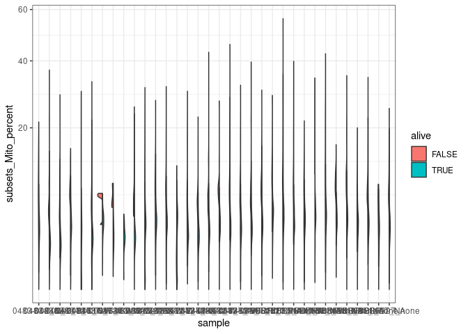
merged_combined_annotation_alive |>

  #violin plot
  ggplot(aes(x=sample, y=subsets_Mito_percent, fill=alive)) +
  introdataviz::geom_split_violin() +
  scale_y_sqrt() +
  theme(axis.text.x=element_text(angle=70, hjust=1)) +
  theme_bw()

## Warning: Groups with fewer than two data points have been dropped.
For each sample according to cell type
#facet by sample, x= celltypes
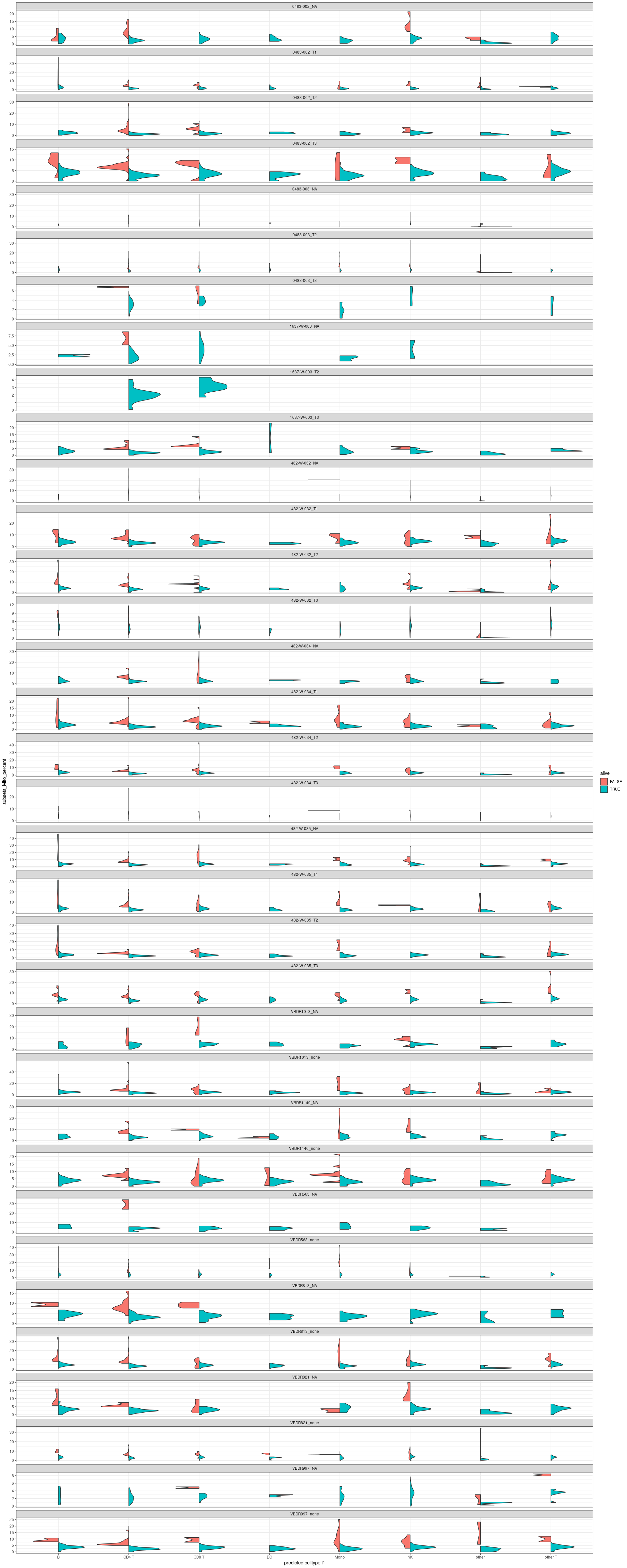
merged_combined_annotation_alive |>

  #violin plot
  ggplot(aes(x=predicted.celltype.l1, y=subsets_Mito_percent, fill=alive)) +
  introdataviz::geom_split_violin() +
  facet_wrap(~sample, scale="free_y", ncol =1) +
  theme(axis.text.x=element_text(angle=70, hjust=1)) +
  theme_bw()

## Warning: Groups with fewer than two data points have been dropped.
## Groups with fewer than two data points have been dropped.
## Groups with fewer than two data points have been dropped.
## Groups with fewer than two data points have been dropped.
## Groups with fewer than two data points have been dropped.
## Groups with fewer than two data points have been dropped.
## Groups with fewer than two data points have been dropped.
## Groups with fewer than two data points have been dropped.
## Groups with fewer than two data points have been dropped.
## Groups with fewer than two data points have been dropped.
## Groups with fewer than two data points have been dropped.
## Groups with fewer than two data points have been dropped.
## Groups with fewer than two data points have been dropped.
## Groups with fewer than two data points have been dropped.
## Groups with fewer than two data points have been dropped.
## Groups with fewer than two data points have been dropped.
## Groups with fewer than two data points have been dropped.
## Groups with fewer than two data points have been dropped.
## Groups with fewer than two data points have been dropped.
## Groups with fewer than two data points have been dropped.
## Groups with fewer than two data points have been dropped.
## Groups with fewer than two data points have been dropped.
## Groups with fewer than two data points have been dropped.
## Groups with fewer than two data points have been dropped.
## Groups with fewer than two data points have been dropped.
## Groups with fewer than two data points have been dropped.
## Groups with fewer than two data points have been dropped.
## Groups with fewer than two data points have been dropped.
## Groups with fewer than two data points have been dropped.
## Groups with fewer than two data points have been dropped.
## Groups with fewer than two data points have been dropped.
## Groups with fewer than two data points have been dropped.
## Groups with fewer than two data points have been dropped.
## Groups with fewer than two data points have been dropped.
## Groups with fewer than two data points have been dropped.
## Groups with fewer than two data points have been dropped.
## Groups with fewer than two data points have been dropped.
## Groups with fewer than two data points have been dropped.
## Groups with fewer than two data points have been dropped.
## Groups with fewer than two data points have been dropped.
## Groups with fewer than two data points have been dropped.
## Groups with fewer than two data points have been dropped.
## Groups with fewer than two data points have been dropped.
## Groups with fewer than two data points have been dropped.
## Groups with fewer than two data points have been dropped.
## Groups with fewer than two data points have been dropped.
## Groups with fewer than two data points have been dropped.
Plot 2 - Visualisation of apoptosis, necrosis, autophagy and stress markers
# selecting stress markers - splitting the markers for better visualisation
stress_markers <- c("JUN", "FOS", "IL6", "TNF", "CXCR4", "SNAI1", "VIM", "GADD45B", "MCL1","STAT1", "IRF7", "IRF3", "IRF1", "CDKN2A", "TP53", "MRTFB", "RBL1", "NUPR1", "IFNG", "IFNB1", "IFNA2", "IFNL1", "IFNA1", "IFNK", "TNF", "IL-12")

#selecting death markers
apoptosis_markers <- c("BCL2L1", "CASP9", "CHP2", "CYCS", "EXOG", "IL1A", "IL1R1", "IL1RAP", "IL3RA", "PIK3CA", "PIK3CD", "PIK3CG", "PIK3R1", "PIK3R2", "PRKAR1B", "NFKBIA", "TNFRSF10A", "TNFRSF10B", "TNFRSF10D", "TNFRSF1A")
necrosis_markers = c("DNML1", "GSDME", "IPMK", "MLKL", "RBCK1", "TICAM1", "YBX3")
autophagy_markers = c("ATG12", "GABARAPL1", "IFNA17", "IFNA8")

#first drop the MT gene from the nCount_SCT :
mitochondrial_genes = grep("^MT-", rownames(merged_combined_annotation_alive[["SCT"]]),value = T)
ribosomal_genes = grep("^RP(S|L)", rownames(merged_combined_annotation_alive[["SCT"]]), value = T)

#remove the gene from the matrix #dim before 98,626 × 29.     98,626 × 29
merged_combined_annotation_alive_no_MT_no_rib <-
  merged_combined_annotation_alive[! rownames(merged_combined_annotation_alive) %in% mitochondrial_genes, ]

merged_combined_annotation_alive_no_MT_no_rib <-
  merged_combined_annotation_alive_no_MT_no_rib[! rownames(merged_combined_annotation_alive_no_MT_no_rib) %in% ribosomal_genes, ]

#re-scaling, see github
all.genes <- rownames(merged_combined_annotation_alive_no_MT_no_rib)
head(all.genes)

## [1] "MIR1302-2HG" "FAM138A"     "OR4F5"       "AL627309.1"  "AL627309.3"
## [6] "AL627309.2"

merged_combined_annotation_alive_no_MT_no_rib<- ScaleData(merged_combined_annotation_alive_no_MT_no_rib, assay = "SCT", slot='scale.data', features = all.genes)

## Warning: The following arguments are not used: slot

## Centering and scaling data matrix

# Creating gene signatures:

# 1 create a gene signature + genes in the signature dataframe:
#stress
stress_markers_df <- as.data.frame(stress_markers)
stress_markers_df$signature <- "stress"
colnames(stress_markers_df)[1] <- ".feature"

apoptosis_markers_df <- as.data.frame(apoptosis_markers)
apoptosis_markers_df$signature <- "apoptosis"
colnames(apoptosis_markers_df)[1] <- ".feature"

necrosis_markers_df <- as.data.frame(necrosis_markers)
necrosis_markers_df$signature <- "necrosis"
colnames(necrosis_markers_df)[1] <- ".feature"

autophagy_markers_df <- as.data.frame(autophagy_markers)
autophagy_markers_df$signature <- "autophagy"
colnames(autophagy_markers_df)[1] <- ".feature"

#bind by rows, obtain only 1 dataframe with all the signatures
gene_signatures <- rbind(stress_markers_df, apoptosis_markers_df, necrosis_markers_df, autophagy_markers_df)


#combine the new dataframe with my seurat object:
#join seurat object with signature dataframe, option long, bind by col created = .features
merged_combined_annotation_alive_no_MT_no_rib_signature <-
merged_combined_annotation_alive_no_MT_no_rib |>
  join_features(
    features = c(stress_markers, apoptosis_markers, necrosis_markers, autophagy_markers),
    shape="long") |>
  left_join(gene_signatures, by = ".feature")

## tidyseurat says: This operation lead to duplicated cell names. A data frame is returned for independent data analysis.

#Plot 1 - facet by gene signatures
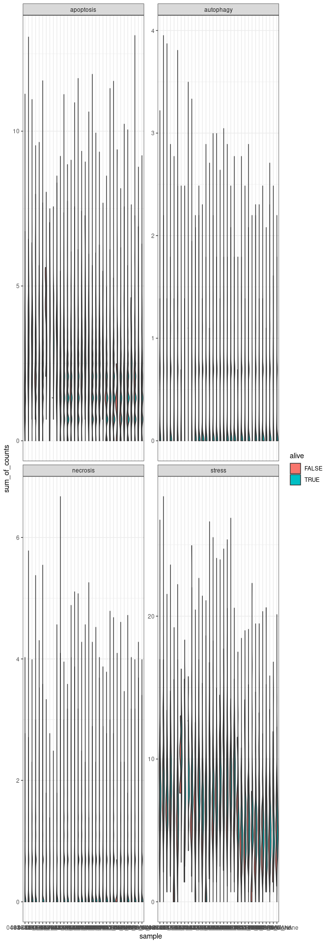
merged_combined_annotation_alive_no_MT_no_rib_signature |>
  group_by(.cell, signature, alive, sample) |>
  mutate(sum_of_counts = sum(.abundance_SCT)) |>
#create the ggplot facet by gene signatures
  ggplot(aes(x=sample, y=sum_of_counts, fill=alive)) +
  introdataviz::geom_split_violin() +
  facet_wrap(~signature,  scale="free_y" ) + #ncol=1
  theme(axis.text.x=element_text(angle=70, hjust=1)) +
  theme_bw()
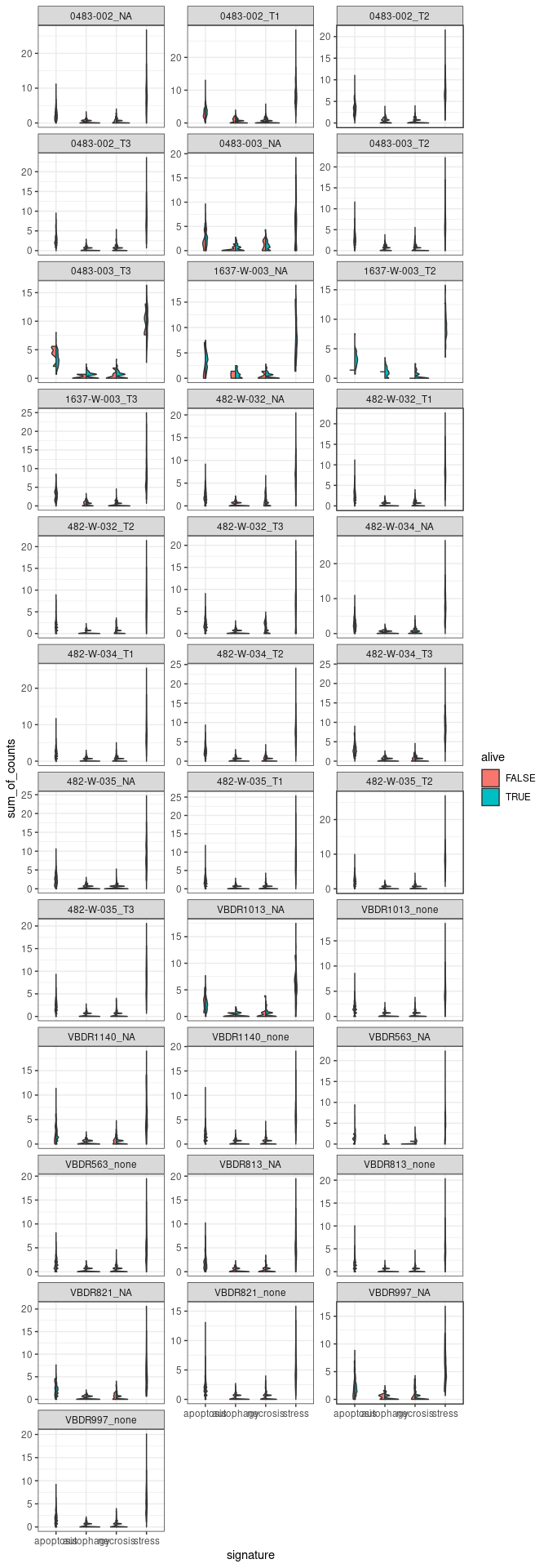
#Plot 2 - facet by samples
#create the column sum of counts
merged_combined_annotation_alive_no_MT_no_rib_signature |>
  group_by(.cell, signature, alive, sample) |>
  mutate(sum_of_counts = sum(.abundance_SCT)) |>

#create the ggplot facet by samples
  ggplot(aes(x=signature, y=sum_of_counts, fill=alive)) +
  introdataviz::geom_split_violin() +
  facet_wrap(~sample, scale="free_y", ncol=3) + #ncol=1
  theme(axis.text.x=element_text(angle=70, hjust=1)) +
  theme_bw()
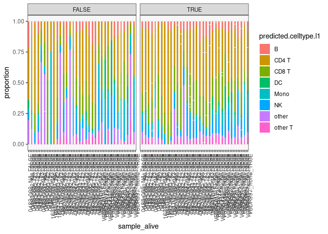
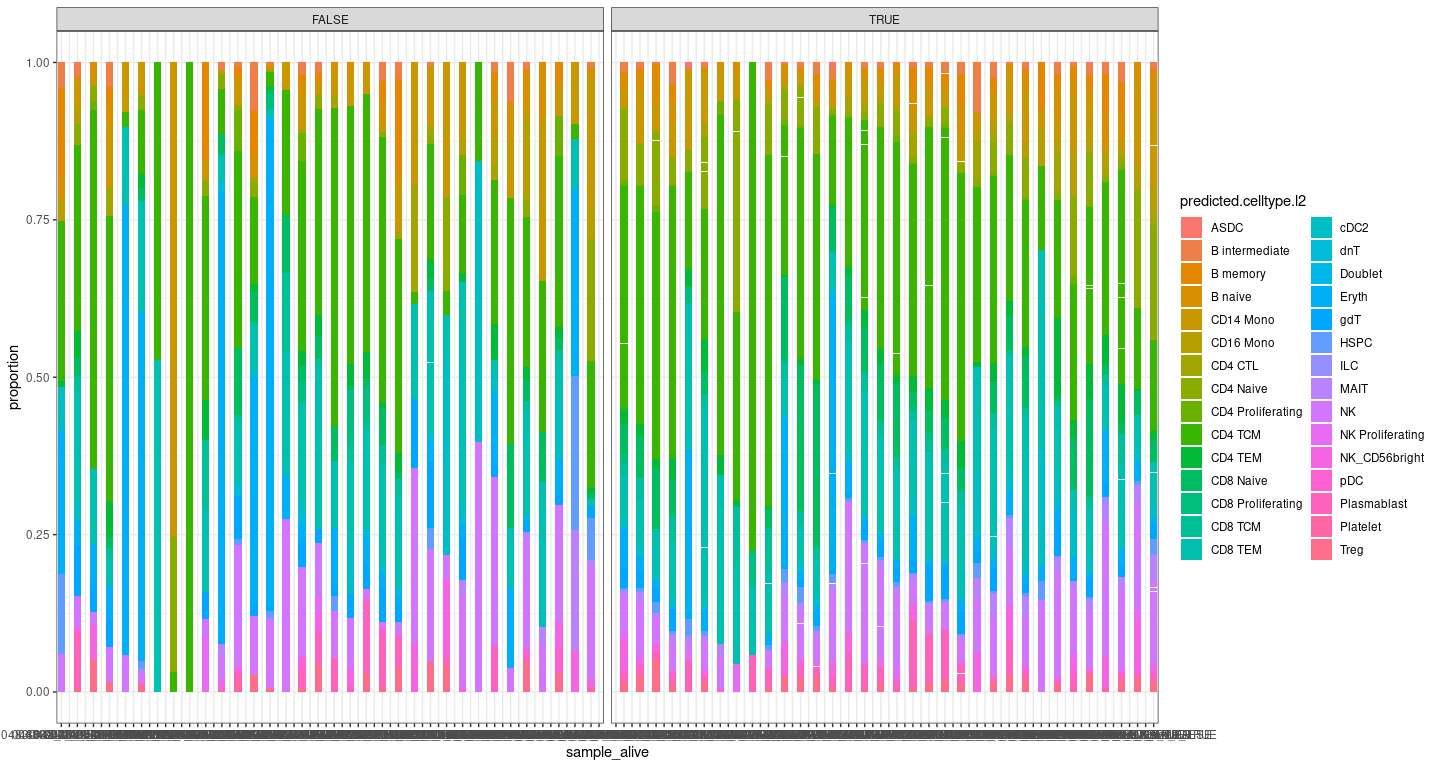
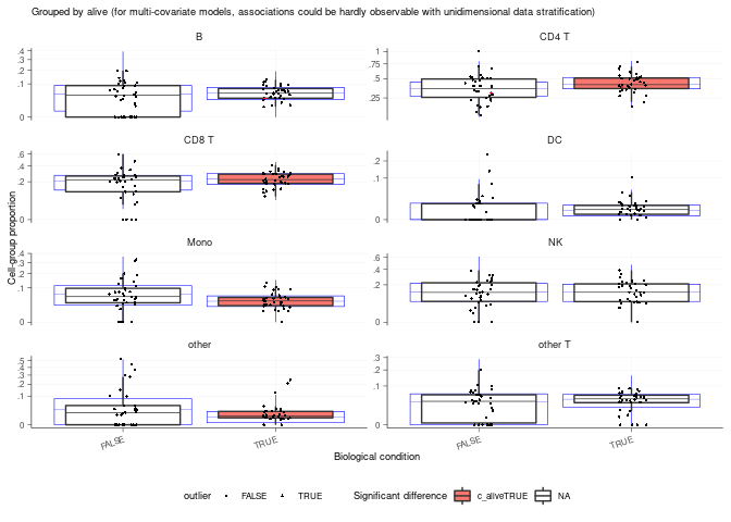
Plot 3 - Composition of cells
## # A tibble: 280 × 9
## predicted.c…¹ param…² covar…³ c_lower c_eff…⁴ c_upper c_pH0 c_FDR count_…⁵
## <chr> <chr> <chr> <dbl> <dbl> <dbl> <dbl> <dbl> <list>
## 1 B (Inter… <NA> -6.91 2.70 9.83 0.312 0.0612 <tibble>
## 2 B aliveT… alive 0.0625 0.233 0.420 0.343 0.0802 <tibble>
## 3 B sample… sample -0.312 0.182 0.571 0.534 0.174 <tibble>
## 4 B sample… sample 0.123 0.706 1.24 0.0398 0.0276 <tibble>
## 5 B sample… sample 0.296 0.821 1.24 0.0125 0.00561 <tibble>
## 6 B sample… sample -3.06 -1.09 0.461 0.134 0.0380 <tibble>
## 7 B sample… sample -5.76 -1.26 -0.748 0 0 <tibble>
## 8 B sample… sample -3.21 -0.455 1.77 0.420 0.121 <tibble>
## 9 B sample… sample -0.820 1.45 3.90 0.157 0.0622 <tibble>
## 10 B sample… sample -0.555 2.90 6.83 0.0503 0.0168 <tibble>
## # … with 270 more rows, and abbreviated variable names ¹predicted.celltype.l1,
## # ²parameter, ³covariate, ⁴c_effect, ⁵count_data
## # ℹ Use `print(n = ...)` to see more rows
## [[1]]
Plot 4 - Check marker for activation induced cell death (Fas/CD95 - FasL/CD95L)
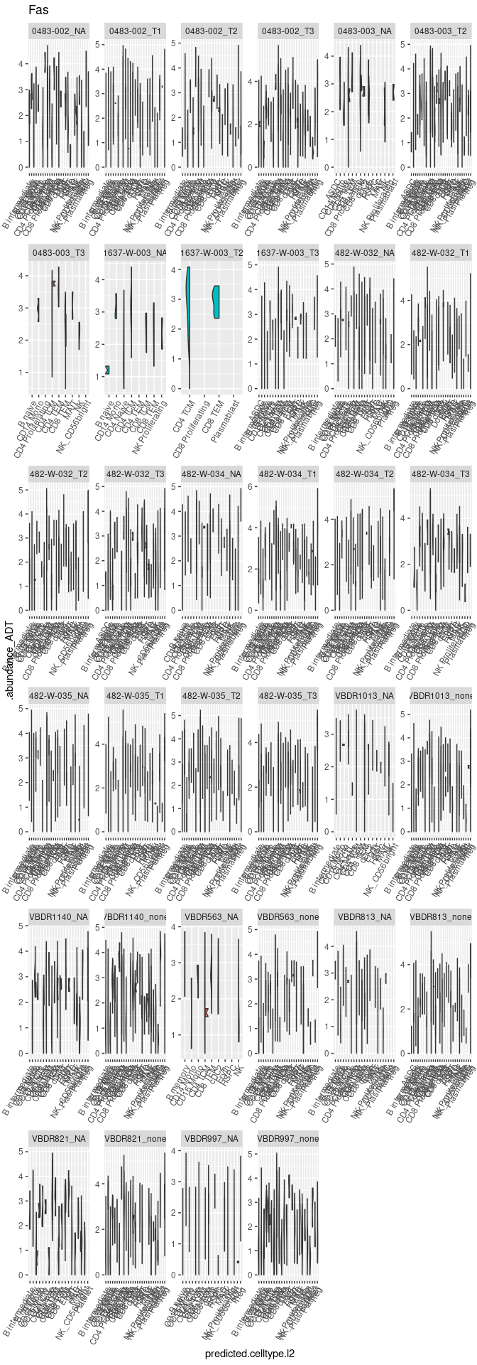
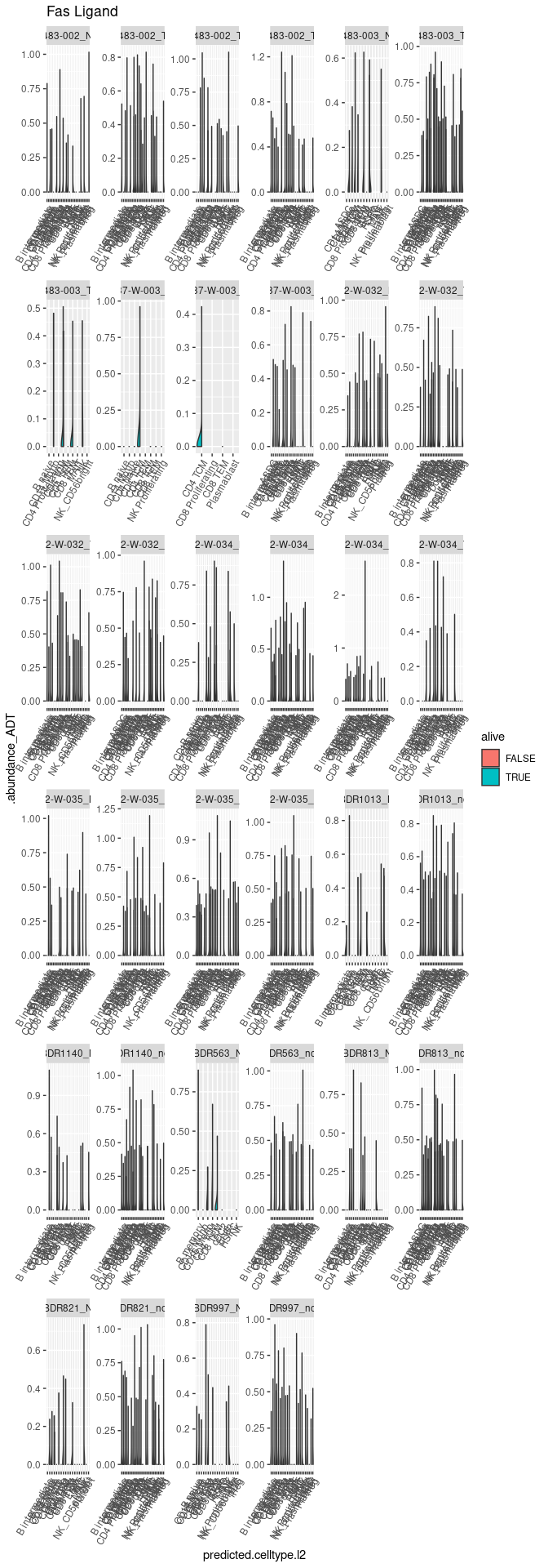
Plot 5 - Gene Ontology genes analysis
## [1] "TRUE" "FALSE"
Gene Ontology: Alive cells
##                p_val avg_log2FC pct.1 pct.2     p_val_adj
## EEF1B2 6.651244e-112  0.5293706 0.978 0.879 2.426706e-107
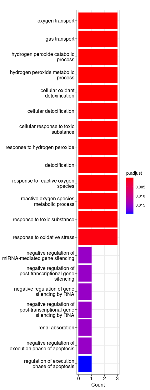
## CCL4    5.375004e-11  0.5896806 0.231 0.172  1.961070e-06
Gene Ontology: Dead cells
##                   p_val avg_log2FC pct.1 pct.2     p_val_adj
## MTRNR2L12 2.903314e-107   1.063250 0.605 0.433 1.059274e-102
## HBB        9.882595e-48   2.254668 0.943 0.935  3.605665e-43
## NEAT1      1.189364e-33   1.175224 0.709 0.658  4.339393e-29
## HBA2       2.424764e-29   2.132526 0.604 0.549  8.846751e-25
## HBA1       1.009746e-20   2.130741 0.408 0.351  3.684059e-16
